
Improve the performance ofcontinuous annealing lines using a predictive control model
Continuous annealing lines are used for heat treatment of cold-rolled steel strip, which is necessary to get the right mechanical properties for various applications. The strip is heated to temperatures between 600 and 800°C by means of radiant tubes in which combustion takes place The steel strip travels in a protective atmosphere of hydrogen and nitrogen to avoid oxidation.
The challenge of this line is to heat up cold-rolled strip to temperatures between 600 and 700°C within tight strip temperature tolerances. Due to strip transitions and enforced speed changes, conventional control has difficulties meeting these tolerances.
A model predictive controller has recently successfully been developed for and implemented in a continuous annealing line with an annual production of 400,000 tonnes. Employing a first-principle furnace model, the controller computes the requires burner load and line speed, such that the coil is annealed at the target annealing temperature while maximizing the line speed and minimizing the transition effects on temperature. In the control algorithm, a nonlinear constrained dynamic optimization problem is solved by applying piecewise linear models over a receding horizon.
The model predictive controller has increased the on-spec strip length from 75 to 98%, while increasing the production capacity by 3% and reducing the natural gas consumption by 6%.
1. Introduction
After cold rolling annealing is necessary to restore mechanical properties before being further processed. In a continuous annealing line the strip is heated to temperatures between 600 and 800°C by means of radiant tubes inside a furnace (RTF). Good control of the annealing process is vital to realise desired product qualities, to maximise process efficiency and line throughput and to minimise energy consumption.
Conventional controllers of these installations do not explicitly consider the effect of furnace thermal inertia and dynamics on the strip temperature. Furthermore, the strip itself disturbs the process each time a welding point, a so-called strip transition, enters the furnace introducing changes in strip dimension, target temperature, speed limit, emissivity, etc. Thus, it is really a challenging task to precisely control the strip temperature in such continuously transitional and time-delay system.
Model predictive control
Model predictive control (MPC) Model Predictive Control (MPC) is a control strategy that uses a model to make on-line predictions of the short term future process behaviour. It optimises the process variables over a particular timeframe in the future. It increases efficiency by pushing the process towards its process constraints without violating them and anticipates on planned process changes, like for example strip transitions and therefore thickness or temperature target changes in a continuous annealing line.
The working principle of MPC can be described with help of Fig. 1.

The dashed blue line shows the predicted output from present into the near future, which is for example the strip temperature in an annealing line. This output is based on constant input presented in the dashed orange line, which is for example the furnace load. This future output can be calculated by means of known future events – such as strip transitions – and an accurate dynamic model. The continuous red line is a constrained process variable, for example a radiant tube safety temperature in continuous annealing. This process variable must not exceed its limits. MPC computes the future inputs, shown as the dotted orange line, to let the controlled output, illustrated with the dotted blue line, match the target as close as possible, without violating the constraints, shown as red dashed lines.
Due to unmeasured disturbances, measurement and model errors, the ‘real’ future will probably deviate from the predicted future. Therefore, only the first manipulation is sent to the process and the measured output is used as new starting point of the next computation.
A first-principle model is preferred over a statistical relation model [1], as the process during the strip transition is strongly non-linear.
Since non-linear models are difficult to implement in the MPC problem [2], piecewise linearization is applied to construct localised linear models that are solved with improved stability. Computational burden is optimised by assigning non-equidistant time steps over the prediction horizon.
2. Rigorous dynamic process model
In the heating section, the strip travels up and down in multiple passes over conveying rolls placed on top and bottom of the furnace (Figure 2). Between the passes, radiant tubes are places which are the energy source. The furnace atmosphere is filled with a protective gas that prevents the strip from oxidation. In the model the furnace is divided into a matrix of computational cells. Depending on the cell position the cell is either a radiant tube cell, a transport roll cell, or an empty cell.

Figure 2 – Radiant tube furnace discretisation into a matrix of cells
Each cell contains a number of elements that represent the wall, the strip, the radiant tube, the gas and/or the roll. Fore each element the heat balances q(T, u) is computed, where vector T represents the temperature states of all elements in the model and vector u contains the process parameters such as the strip thickness and width, the line speed and the furnace heating power.
The dynamic solution is based on numerical integration of the following non-linear partial derivative function.

The partial net heat flow function qi for the element i depends solely on the temperature states T and process parameters u. The element mass m is constant, except for the strip element and the specific heat cp depends on the material and temperature of the element.
The rigorous model structure is chosen as such that the temperature derivative T, gradient T∇ and u∇ are computationally cheap (see Equation 2, where fn(T,u) is the rigorous model).
![]()
The gradients are useful for stabilizing the dynamic solution and for finding the steady state solution0=dtdT, which is used as the initial state for the calculation.
Radiation heat transfer
In the radiant tube furnace about 95% of the heat is transferred by radiation and therefore an accurate model description of the radiation heat transfer is vital for this controller. The radiation heat transfer is based on the method of computing the total exchange of radiation within an enclosure described by [3], where the gas is assumed to be transparent.
The view factors depend on the geometry of the considered cell and are calculated using standard geometrical equations [4]. The geometry of the tube cell is shown in Figure 3.

Figure 3 – Different elements within the RTF cell
Heat transfer from tube
The radiant tube with attached burner in Figure 4Figure 5 is the energy source of the furnace. The combustion takes place inside the tube on the burner end. Hot flue gases travel though the W-shape tube and exit at another end. A recuperator is attached to the flue gases exit to recover the waste heat for preheating the combustion air.

Figure 4 – Schematic layout of radiant tube unit with burner and recuperator
The heat balance computation of the tube consist of:
- •Combustion heat
- •Heat recovery by the recuperator
- •Radiation from the flue gasses to the radiant tube inner surface
The last term forms the boundary for the furnace radiation calculation.
Other heat transfer
Besides radiation and the tube heat balance, other heat transfer principles take place in the furnace and are thus modeled in the rigorous dynamic model, such as:
- •Convective heat transfer between gas and surface elements
- •Heat extraction due to protective gas movement.
- •Heat extraction due to strip movements
- •Heat loss and storage at the refractory by means of conduction
- •Heat transfer between the strip and the conveying rolls
Model validations
The line has a radiant tube furnace with 148 radiant tubes located in 5 heating zones. The model is configured accordingly and has a total of 772 elements (or temperature states).
The two graphs plot in Figure 5 the model output in comparison with the measurements. It shows overall a good agreement between the calculated and measured values, with an average prediction error of 14°C for the zone temperature and 8°C for the strip temperature. Furthermore the model predicts the process dynamics quite accurate, for instance at the thickness transition at 3:50 and the speed changes at 1:30 and 11:10. The results prove that the model captures the process dynamics sufficiently accurate.

Figure 5 – Model validation results
3.Model Predictive Control
Prediction model
The non-linear rigorous model explained in the previous chapter cannot directly be applied in MPC. Therefore it computes a set of piecewise linear state space models along a prediction horizon [5] (see Equation 3).
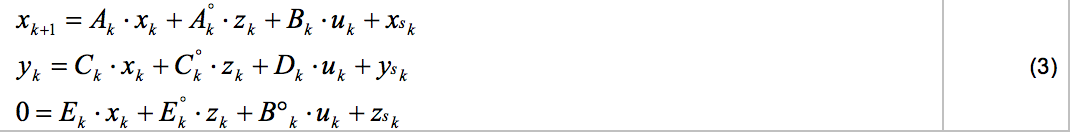
Where xk is the state (or temperature) vector, uk is the system input vector (line speed and zone load), and yk is the system output vector with the strip and zone temperatures. The algebraic term z captures the steady state elements (the gas elements). The terms xs, yz and zs are introduced to enable the linear model to operate in absolute scale without loss of generality and accuracy and allow performing linearization in a transient point of operation.
Figure 6 shows the result of the strip temperature response to a step change in the line speed for the single linear model compared to the non-linear model. The linear model predicts the temperature response sufficiently accurate, where only a small offset is visible at the end.

Figure 6 – Temperature response to a speed perturbation from 600 m/min to 450 m/min of the linear model versus the non-linear rigorous model
Time step size
Large time steps are desired to limit the computational burden; however sufficient detail in the short term and during transitions is required. Using the Tustin transformation [6], the prediction horizon can be filled with different time step size models, allowing sufficient detail where needed. This is illustrated in Figure 7, which shows that more detail is placed in the first few time steps and around a transition. The final time step stretches up to the end of the prediction This distribution is computed for every control step to capture and follow closely the approaching transition.

Figure 7 – Adaptive time step distribution in prediction horizon
Kalman filter
The rigorous dynamic model is used as the state observer, where an extended Kalman filter [6] is applied to estimate the temperature state and model parameters. This ensures that the rigorous dynamic model follows the measurements closely.
Constrained optimization problem
The objective function describes mathematically the optimisation problem and for the continuous annealing the main objective is to achieve the annealing target temperature and maximise the throughput. Stable operation and energy conservation are considered as the secondary objectives.
Constraints are considered explicitly in the optimization, where the installation constraints like actuator ranges and design maximum speed are considered as ‘hard limitations’. These hard constraints need to be fulfilled anytime to avoid ‘unrealistic’ control actions. The process constraints are considered as ‘soft constraints’, like furnace safety temperature, where a violation of the soft constraints is penalised in the objective function allow the controller to recover from undesired situations.
4. Implementation
Production trials were executed and showed that MPC consistently outperformed the conventional control and achieved broad improvements. The strip temperature was very accurately controlled, even at strip transitions as shown in Figure 8. Anticipated actions for both line speed and furnace load result in very small off-spec lengths at transitions, for example when the strip thickness changes from 0.24 to 0.19 mm as illustrated in Figure 8.

Figure 8 – An example of strip transition control by the MPC-based controller
A two-month endurance trial was executed to judge the performance of the new controller against the conventional control. The evaluation results as shown Figure 9 revealed that the amount of strip length within the target temperature range improved from 75% to 98%. On top of that the production rate increased by 3%, while the natural gas consumption decreased by 6%. The latter benefits were obtained because the model predictive controller was not only challenged to reduce the strip temperature error, but also to maximise production speed and to minimise gas consumption. Furthermore due to more stable operation, the number of line stops where significantly reduced. The furnace operators are delighted with the new furnace controller, among others because the amount of required operator interventions has decreased significantly.

Figure 9 – Improvement in strip temperature control accuracy due to Model Predictive Control
5. Conclusions and outlook
The in-house developed model predictive control system has increased the on-spec length from 75 to 98%, while increasing the production capacity by 3%, and reducing the natural gas consumption by 6% and operator intervention to minimum.